


.png?width=400&height=400&ext=.png)
What is an ESAL? Guide to equivalent single axle load
by Andrew Lees, on May 16, 2024
The relationship between axle load and pavement damage is exponential: a single 80kN axle causes over 3000 times more damage than a single 8kN axle. Equivalent single axle load (ESAL) provides a means by which the accumulative traffic load on a road pavement, resulting from multiple vehicle types with different axle configurations, can be expressed as a number of passes of a standard axle load.
Figure 1 - Trucks in Michigan are allowed a higher gross weight than in other States - But with more axles to keep axle loads down (Source DAT)
The cumulative effect of multiple vehicle passes is a crucial input into pavement design. The use of ESALs allows mixed traffic loading to be entered into a pavement design calculation as a single representative number. By representing the damaging effect of vehicles with widely differing weights and axle configurations, we are able to design long lasting roads that meet society’s needs.

This load equivalency approach, where each class of vehicle is assigned a damage factor to convert its load effect to a number of equivalent passes of a standard axle, arose from a major series of road trials known as the AASHTO Road Test and published by the Highways Research Board in 1962.
In this article we will look at how traffic load is represented using ESALs and how this is incorporated into road pavement design. We will also look at UK pavement design practice and why it uses a variant to ESALs.
There’s plenty to go through here. If you’re interested in a particular section, use the links below to navigate to it:
- What is an ESAL?
- How are ESALs expressed?
- How is ESAL used?
- No ESALs in the UK?
- The importance of ESAL in designing pavements
- Key factors that influence ESAL
- How to calculate ESAL for design
- Important considerations for estimating design traffic
- Pavement performance and load equivalency factors
- How is design traffic calculated in the UK?
- Tensar Solutions
'Andrew Lees returns to our screen for the latest episode of Ask Andrew in Ho Chi Minh City in Vietnam, where he explains what an Equivalent Single Axle Load is.
What is an ESAL?
An ESAL, or equivalent single axle load, represents the damage effect from a single pass of a standard axle load. The damage effect of any vehicle can be expressed in terms of ESALs – the specific number of passes of a standard axle that would cause the equivalent damage as a single pass of the vehicle.

Figure 2 - Photo demonstrating an example of asphalt layer rutting
What is the difference between ESAL and axle load?
Different road vehicles have different loaded weights and different axle configurations. On any one vehicle, the load is not distributed equally across all axles. This makes it difficult to input true axle loading from a mix of vehicle types over time in any road design. It is far easier if we can convert all vehicles passing to an equivalent number of passes of a standard axle load. For this we use ESAL – equivalent single axle load, representing the damage effect of a single pass from a standard axle.
In road pavement design, we are not interested in the total number of vehicles or even the sum of all axle loads, we want to know the cumulative damage caused by the mix of vehicles over time. We need to convert the damage effect from each vehicle type to the number of standard axle passes that would generate an equivalent damage effect. For each vehicle type (with specific loading and axle configuration) we determine its equivalent single axle load (ESAL). It is then a simple matter to calculate the cumulative traffic effect over time in terms of ESALs.
Significantly, the damage effect is not linearly proportional to the weight of a vehicle. One 40 tonne vehicle does significantly more damage than four 10 tonne vehicles. The conversion of actual axle load (a function of vehicle load and axle configuration) to ESALs must take account of this. More on this later.
Michigan trucks – Higher gross weight but lower axle load
The state of Michigan is unique in allowing gross vehicle weights of 164,000lbs. This contrasts with the normal maximum of 80,000lbs in other states. Michigan trucks avoid causing excessive pavement damage by increasing the number of axles (see Figure 1) . In fact, the average axle load is lower for Michigan trucks than conventional trucks elsewhere. Maximum axle load is limited to 13,000lbs in Michigan compared to 18,000lbs in other States.
How are ESALs expressed?
ESALs are considered to be a ratio of the number of passes of a standard axle divided by the number of passes of a specific vehicle that would cause the same pavement damage. Damage may be measured as a change in the Pavement Serviceability Index (PSI). The standard axle load used by different road authorities varies. In the US and UK it is 80kN.
ESALs are calculated by applying load equivalency factors to the estimated commercial traffic flow (see below). Significantly, the load equivalency factors applicable to each category of commercial vehicle are not uniform across all regions, or for different pavement type and structure. Regional road authorities determine load equivalency factors that represent the predicted local commercial traffic fleet. Because of this, design traffic (ESALs) calculated for a commercial traffic flow in one region may not be the same as that calculated for the identical traffic flow in another region.
For permanent roads, the design traffic (or design life) can be expressed in terms of total ESALs. The number will be large, so it is sometimes convenient to use units of million ESAL. This unit can be written in different ways, with different road authorities using different acronyms, such as million single axle load (MSAL), or million standard equivalent axles (MSEA).
How is ESAL used?
Traffic comprises a mix of vehicle types. Commercial vehicles have different loading and axle configurations. Any pavement design must take account of the damaging effect of each type of vehicle. One way to do this that is simple and effective is to use load equivalency, where specific vehicle types are converted to ESALs.
The ESAL approach represents pavement deterioration due to the repeated passage of traffic. There are other deteriorating effects, such as ageing of the asphalt that are time and climate dependent, but the service life will primarily be defined in terms of the design traffic – the cumulative traffic effect. This is expressed in terms of total number of ESALs.
No ESALs in the UK?
The UK Design Manual for Road and Bridge Works does not use the term ESAL. The effect of traffic and vehicle loading on pavement design is still based upon load equivalency, converting the vehicle load to an equivalent number of standard 80kN axle passes, but the methodology differs, and design traffic is expressed at million standard axles (msa). More on this later.
The importance of ESAL in designing pavements
From the first day open to traffic, every road is deteriorating towards failure. Each passing of a vehicle causes damage to the road pavement. The magnitude of damage from a single vehicle may be small, but the cumulative damage effect from the passage of multiple vehicles will ultimately determine the service life of the pavement. The cumulative damage effect can be defined in terms of ESAL. The service life of the pavement will be expressed in terms of design traffic, the total number of ESALs before serviceability limits are reached. All good pavement design must balance the whole life cost vs design life (ESALs). This usually involves a more complex balance to minimise construction cost and maintenance costs, while maximising design life.
Key factors that influence ESAL
As we have discussed above, ESAL represents the damage effect of the passing of a standard axle. It is not a simple count of axles or vehicles passing. To calculate the ESALs for a new or reconstructed road we need to know about the mix of traffic, the initial traffic volume and predicted growth, the road type, and number of lanes. The conversion of vehicle load to ESALs is dependent upon pavement type (rigid or flexible) and pavement structure (strength and stiffness).
Initial traffic count
This can be measured or estimated from existing traffic data to determine the average annual daily flow. The count needs to provide numbers and information on the mix of commercial vehicle types. Private cars and small vans (with an unladen weight of 1.5T or less) are discounted as they have only a minor influence on pavement life. A fully loaded minivan will only equate to 0.003 ESALs.
Traffic period
Although design life will be expressed in terms of ESALs, the highway engineer will need to know the client's requirement for the target service period for the road. For major roads this might be 40 years.
Traffic growth
To estimate the total ESALs over the design period, the forecast traffic growth rate must be considered. Regional road authorities will each have their own growth forecasts for different road categories and locations.
Load equivalency factor
The relationship between axle load and pavement damage is not linear but exponential. Axle configuration also has a major influence. A single 80kN axle causes over 3000 times more damage than a single 8kN axle. A single axle does 11 times more damage than a dual axle carrying the same load. The use of load equivalency factors applied to each class or category of commercial vehicle will adjust for this. Regional road authorities will have determined load equivalency factors to be applied in their region when calculating design traffic in ESALs.
The AASHTO (1993) method uses load equivalency factors to convert axle load into a change in Pavement Serviceability Index (PSI) equivalent to that produced by a single pass of a standard 80kN axle. The factors were derived from the AASHTO Road Test (see above), but modified to include additional axle configurations. The type of pavement, (whether rigid or flexible), the pavement structure (defined by structural number for flexible and slab thickness for rigid), and the design serviceability (the required PSI at end of service life), all influence the load equivalency factors.
Other roads authorities use differing approaches to derive load equivalency factors.
Lane distribution
For carriageways with 2 or more lanes in one direction, commercial vehicle traffic will be distributed across lanes. The greater proportion will be on the inner lane, but this will vary with vehicle flow. Regional road authorities will have guidelines for estimating the proportion of commercial traffic in each lane. This has an influence of the design traffic (ESALs).
How to calculate ESAL for design
Most pavement design methods require an estimate to be made of the design traffic loading over the design period. Different road authorities have their own approach, but many follow the load equivalency approach converting mixed traffic to an equivalent number of standard axle passes.
Estimation of design traffic will be based upon:
- Target design period
- Initial traffic count
- Forecast commercial vehicle growth
- Lane distribution factor
- Commercial vehicle mix by class
- Load equivalency factor (or wear factor) for each vehicle class
As we learned above, the AASHTO 1993 method uses load equivalency factors (damage factors) to convert commercial traffic load into the number of equivalent single axle loads that would generate the same damage – as measured by a change in the Pavement Serviceability Index (PSI). An approach for this is set out in “AASHTO Design Guide 1993 Appendix D - Conversion of mixed traffic to equivalent single axle loads for pavement design”.
The AASHTO 1993 procedure involves:
- Derivation of load equivalency factors
- Conversion of mixed traffic to equivalent single 80kN axles passes
- Consideration of lane distribution effects
Load equivalency factors – AASHTO 1993 - Appendix D includes axle load equivalency factor tables for a range of pavement structures, axle configurations and terminal serviceability. To use the tables, it is first necessary to assume a structural number (SN) for flexible pavements or slab thickness (D) for rigid pavements. The guide suggests that a SN of 50 or a D of 9in will normally give results sufficiently accurate for initial design purposes. If the resulting pavement design is different from that initially assumed, an iterative process should then be undertaken to reach a final design.
Growth factors – AASHTO 1993 – Appendix D Table D20 provides multipliers for a given growth rate and design period. Growth normally varies between vehicle types. Regional Authorities need to determine appropriate growth rates based on local knowledge and development plans.
Lane distribution - AASHTO 1993 - Appendix D suggests that local road authorities determine lane distribution factors based on traffic measurement data. However, the typical range of factors used by a number of US State Highway Authorities is provided.
Table 1 - Typical Lane distribution factors (source AASHTO 1993 - Appendix D)
| Number of Lanes in both directions | Percent of ESAL traffic in Design Lane |
| 1 | 100 |
| 2 | 80-100 |
| 3 | 60-80 |
| 4 or more100 | 50-75 |
A general equation for calculating the traffic load in total ESALS for each category of axle load is given below. The Design traffic in ESAL will be the sum of traffic load calculated for each traffic category.
Traffic Load for Axle Category i (ESALs) = fd.Grn.Ti.fL
Traffic load for axle category i (ESALs) = fdGrnTiNifl
Where:
fd =lane distribution factor (obtained from Regional Road Authority – regional specific)
Grn =traffic growth factor for design period n years (obtained from Regional Road Authority location specific)
Ti =initial average annual daily traffic flow for axle category i in one direction (from traffic counts or estimated)
Ni =number of axles for vehicle in category i
fL =load equivalency factor for vehicle category i (defined by Regional Road Authority – regional specific)
It is clear that many of the factors used in the above calculation are to be obtained from the regional road authority. They are based on locally obtained data and influenced by local factors. It is important to use factors appropriate to the location of the project.
Most road authorities have simplified the process by publishing truck equivalency factors to convert vehicle types in a traffic mix into ESALs. These factors provide only estimates if applied to roads other than those for which the data was obtained.
Important considerations for estimating design traffic
The estimation of design traffic (total ESALs) relies on multiple estimated inputs. The result is sensitive to the estimated growth rate for each traffic category plus the load equivalency (damage) factors assumed. The input of professional traffic engineers is advised for all complex or larger schemes.
Estimated growth
While regional road authorities provide growth rates that may be applied regionally, the highway engineer must consider whether local commercial or industrial development or the opening of local connecting roads will skew the growth and traffic mix.
Load equivalency factors
Wear or damage factors are based upon historical performance data. Major climate change related effects may impact future performance. Events such as flooding may become more prevalent, severely impacting pavement performance and service life.
Lane distribution
Future developments in traffic management, such as automated truck convoys, could drastically change the distribution of commercial traffic across lanes.
Pavement performance and load equivalency factors
The service life of any pavement will be limited by the cumulative damage from traffic. Each vehicle pass adds incrementally to the cumulative damage. What are the mechanisms and nature of that damage?
In flexible pavements, there are a range of factors affecting deterioration but fatigue of the asphalt as a result of traffic loading plays a significant role. As the asphalt flexes under the action of traffic, the lateral strain at the bottom of the asphalt layer initiates cracking, which develops into fatigue cracks that can penetrate upward to the surface. At that point, the pavement has failed. This is often evident by alligator type cracking in road surfaces (see figure below). Thicker asphalt will reduce the strain at the base, delaying the initiation of cracks, and also prolonging the propagation crack to the surface.
.jpg "fatigue-cracking-(1).jpg")
Figure 3 - Severe fatigue cracking due to subgrade softening resulting from poor drainage.
Flexing of the asphalt layer is directly influenced by the support provided by the unbound layers beneath. A strong base layer distributes load down through the subbase and into the subgrade with minimal vertical deformation, both elastic and permanent. Small deformations mean minimal flexure in the asphalt, reducing the fatigue effect. The strength and stiffness of unbound layers can be increased by increasing layer thickness, or alternatively by mechanical stabilisation using a stabilisation geogrid, such as Tensar InterAx.
Weak subgrade soils can also contribute to pavement deterioration. Permanent deformation in the subgrade increases flexure of the asphalt layer above. Mechanical stabilisation of the subbase using Tensar InterAx geogrid can overcome soft ground problems.
How is design traffic calculated in the UK?
ESALs are not used in the UK Design Manual for Roads and Bridges. However, the load equivalency approach, developed from the AASHTO road test (1962) remains the basis of the method used. Vehicle loads are converted to a number of equivalent standard 80kN axles. This is done by applying a wear factor. Each class of vehicle is assigned a wear factor, calculated from vehicle loads measured using weigh-in-motion sensors on the UK road network. Guidance is provided in CD 224 – Traffic Assessment.
Vehicle classification
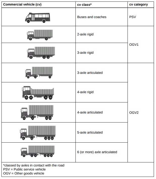
CD 224 defines eight classes or commercial vehicles, grouped into three categories. See below.
Figure 4 - Commercial Vehicle Classes and Categories (source Design Manual for Roads and Bridges - CD 224 Traffic Assessment))
Wear factors
CD 224 provides wear factors for each class and category of vehicle. There are different wear factors for use with new road design and road widening (WN), and for maintenance of existing roads (WM). See below.
4th Power law for wear – In the UK and many other countries, structural wear for pavement design is taken as being proportional to the 4th power of the axle load.
Table 2 - Wear factors for commercial vehicles - (source CD 224)
| Vehicle Class & category | Maintenance WM | New WN |
| Buses & coaches | 2.6 | 3.9 |
| 20-axle rigid | 0.4 | .06 |
| 3-axle rigid | 2.3 | 4.6 |
| 3 and 4-axle articulated | 1.7 | 2.5 |
| 5-axle articulated | 2.9 | 4.4 |
| 6-axle articulated | 3.7 | 5.6 |
| OGV1 + PSV | 1.3 | 1.9 |
| OGV2 | 3.2 | 4.9 |
| All commercial vehicles (70% OGV2) | 2.7 | 4.0 |
Growth factor
CD 224 provides growth factors (G) for future traffic. The factors are based on UK traffic forecasts as are specific to UK use.
Table 3 - UK Growth factors (G) for future traffic (Source CD 224)
| Design period (years) | 5 | 10 | 15 | 20 | 25 | 30 | 35 | 40 |
| OGV1 + PSV | 1.02 | 1.05 | 1.05 | 1.11 | 1.14 | 1.17 | 1.21 | 1.24 |
| OGV2 | 1.04 | 1.1 | 1.16 | 1.23 | 1.30 | 1.37 | 1.46 | 1.54 |
| All commercial vehicles | N/A | 1.45 | ||||||
Lane distribution
The percentage of commercial vehicles using each lane is dependent on the number of lanes. CD 224 provided a recommendation for the proportion (P) of commercial vehicles in the most heavily trafficked lane and also for the lesser trafficked lanes. The values for the heavily trafficked lane are shown below.
Table 4 - Assumed proportion of commercial vehicles in the most heavily loaded lane (Source CD 224)
| Number of lanes in one direction | Flow (F) commercial vehicles per day | P% |
| 2 or 3 | <5,000 | P=100-0(0.0036 x F) |
| 5,000 - 25,000 | P = 89-(0.0014 x F) | |
| >25,000 | P = 54 | |
| 4 or more | <10,000 | P = 100-(0.0036 X F) |
| 10,000 - 25,000 | P = 75(0.0012 X F) | |
| >25,000 | P = 45 |
The calculation for design traffic in million standard axles (msa) is as follows:
The first step is to calculate the weighted annual traffic (Tc )
Tc = 365 .F. G.10-6msa
Next, the Design traffic (T) is calculated.
T = ∑ Tc. Y .P
Where:
Tc Weighted annual traffic for commercial vehicle category c
F Commercial vehicle flow
G Growth factor
W Wear factor (or damage factor)
Y Design period (years)
P Percentage of commercial vehicles in heaviest loaded lane
T Design traffic (ESALs)
Example calculation of design traffic (using CD 224 for UK)
A new 2-lane dual carriageway is to be constructed with a design period of 40 years. The initial total daily flow of commercial vehicles is estimated to be 3,000, of which 60% are category OGV2 commercial vehicles and 40% OGV1 and PSV combined.
| Commercial vehicle category | Average annual daily flow (F) | Growth factor (G) for 40 years (from CD 224) | Wear Factor (W) | Weighted annual traffic (Tc) |
| Wn from CD 224 | ||||
| OGV1 + PSV OGV2 |
40% x 3000=1200 60% x 3000=1800 |
1.24 1.54 |
1.9 4.9 |
1.01 4.84 |
| Total daily flow of commercial vehicles | 3000 | Total weighted annual traffic ∑Tc |
5.85 | |
| Percentage of vehicles in heaviest lane (P) from CD 224 | 89.2% | |||
| Design period (Y) | 40 years | |||
| Design traffic (T) | 229.7 msa | |||
The calculated design traffic is 223 msa.
Tensar solutions
Pavement design, whether empirical or mechanistic-empirical, will output a design life for the pavement in ESALs. This needs to be equal to or greater than the design traffic ESALs.
For flexible pavements, the design life can be extended by the incorporation of a stabilisation geogrid such as Tensar InterAx geogrid. The effect of the geogrid is to confine the aggregate particles, restricting rotation and movement of the particles under the action of repeated traffic loads. This increases the strength of the unbound layers, which in turn improves support to the surfacing layers. The result is an extension to service life. For more information on pavement improvement see our webinar, Improving the Performance of Flexible Pavement with Tensar Geogrid or speak to our team today.
The beneficial effect of Tensar mechanical stabilisation on pavement performance and the increase in pavement life (in ESALs) is illustrated in the four figures below.

Figure 3 - Conventional pavement design for Design Life 1 million ESALS

Figure 4 - Tensar mechanically stabilised option 1 - marginal increase in life for lower Initial cost.

Figure 5 - Tensar mechanically stabilised option 2 - Extended design life for the same initial cost.

Figure 6 - Tensar mechanically stabilised option 3 - Extended life with lowest whole-life cost.